Backpropagation Step by Step

If you are building your own neural network, you will definitely need to understand how to train it. Backpropagation is a commonly used technique for training neural network. There are many resources explaining the technique, but this post will explain backpropagation with concrete example in a very detailed colorful steps.

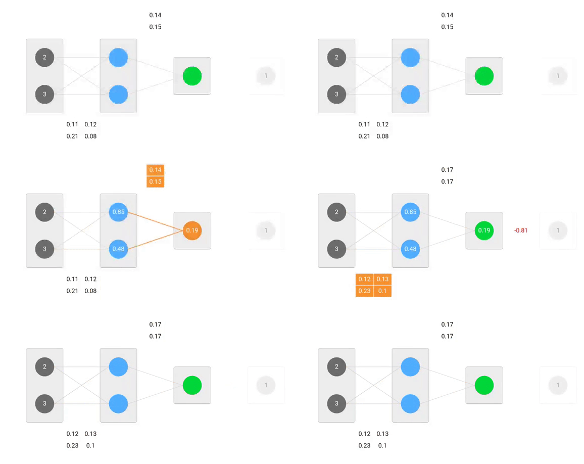
You can see visualization of the forward pass and backpropagation here. You can build your neural network using netflow.js

Overview

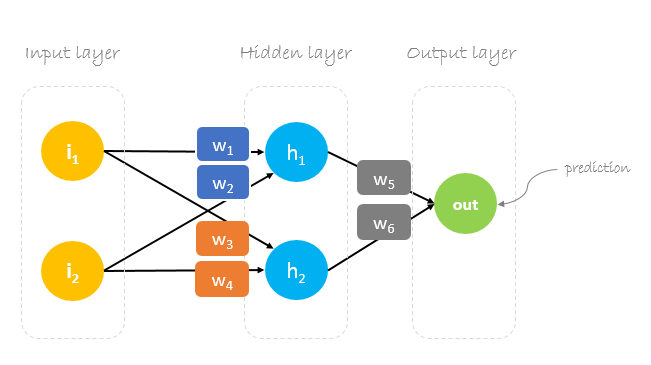
In this post, we will build a neural network with three layers:

• Input layer with two inputs neurons
• One hidden layer with two neurons
• Output layer with a single neuron

Weights, weights, weights

Neural network training is about finding weights that minimize prediction error. We usually start our training with a set of randomly generated weights.Then, backpropagation is used to update the weights in an attempt to correctly map arbitrary inputs to outputs.

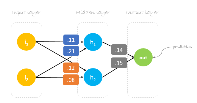
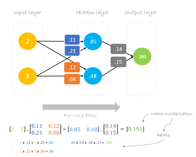
Our initial weights will be as following: w1 = 0.11, w2 = 0.21, w3 = 0.12, w4 = 0.08, w5 = 0.14 and w6 = 0.15

Dataset

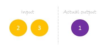
Our dataset has one sample with two inputs and one output.

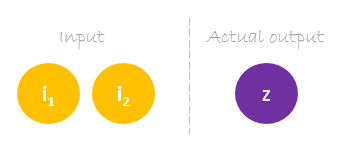
Our single sample is as following inputs=[2, 3] and output=[1].

Forward Pass

We will use given weights and inputs to predict the output. Inputs are multiplied by weights; the results are then passed forward to next layer.

Calculating Error

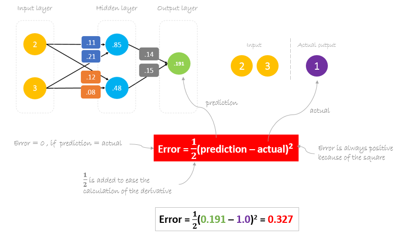
Now, it’s time to find out how our network performed by calculating the difference between the actual output and predicted one. It’s clear that our network output, or prediction, is not even close to actual output. We can calculate the difference or the error as following.

Reducing Error

Our main goal of the training is to reduce the error or the difference between prediction and actual output. Since actual output is constant, “not changing”, the only way to reduce the error is to change prediction value. The question now is, how to change prediction value?

By decomposing prediction into its basic elements we can find that weights are the variable elements affecting prediction value. In other words, in order to change prediction value, we need to change weights values.

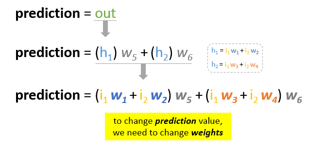
The question now is how to change\update the weights value so that the error is reduced?
The answer is Backpropagation!

Backpropagation

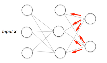
Backpropagation, short for “backward propagation of errors”, is a mechanism used to update the weights using gradient descent. It calculates the gradient of the error function with respect to the neural network’s weights. The calculation proceeds backwards through the network.

Gradient descent is an iterative optimization algorithm for finding the minimum of a function; in our case we want to minimize th error function. To find a local minimum of a function using gradient descent, one takes steps proportional to the negative of the gradient of the function at the current point.

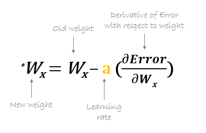
For example, to update w6, we take the current w6 and subtract the partial derivative of error function with respect to w6. Optionally, we multiply the derivative of the error function by a selected number to make sure that the new updated weight is minimizing the error function; this number is called learning rate.

The derivation of the error function is evaluated by applying the chain rule as following

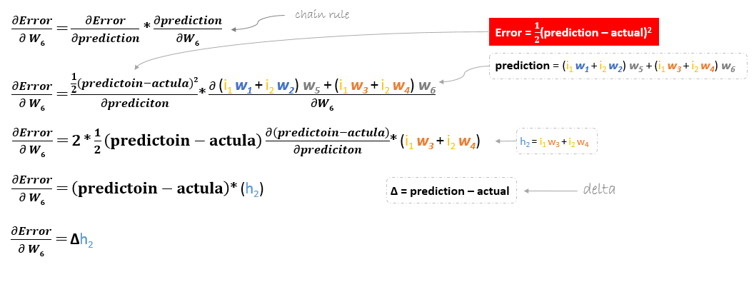
So to update w6 we can apply the following formula

Similarly, we can derive the update formula for w5 and any other weights existing between the output and the hidden layer.

However, when moving backward to update w1, w2, w3 and w4 existing between input and hidden layer, the partial derivative for the error function with respect to w1, for example, will be as following.

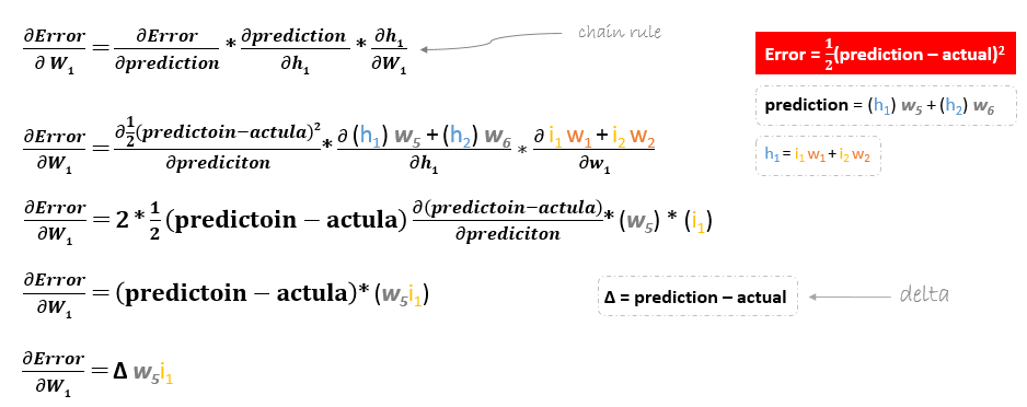
We can find the update formula for the remaining weights w2, w3 and w4 in the same way.

In summary, the update formulas for all weights will be as following:

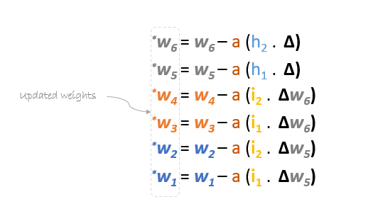
We can rewrite the update formulas in matrices as following

Backward Pass

Using derived formulas we can find the new weights.

Learning rate: is a hyperparameter which means that we need to manually guess its value.

Now, using the new weights we will repeat the forward passed

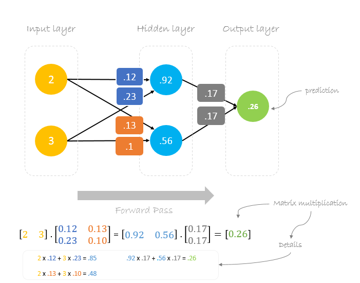
We can notice that the prediction 0.26 is a little bit closer to actual output than the previously predicted one 0.191. We can repeat the same process of backward and forward pass until error is close or equal to zero.

Backpropagation Visualization

You can see visualization of the forward pass and backpropagation here.

You can build your neural network using netflow.js